Unlike a SaaS or retail model, your outputs here depend on reserve data quality, decline curve assumptions, and commodity price scenarios you can't control. That's the exact spot where analysts coming from other sectors get stuck.
This guide walks through what the model involves, how to build one step-by-step in Excel, its four core components, its four types by industry vertical, and the mistakes that most often derail accuracy.
Key Takeaways
- Depleting reserves, volatile prices, and units like Bbl, Mcf, and BOE set oil & gas models apart
- Four core components drive every model: revenue, cost, production, and valuation
- Valuation method must match the vertical: NAV for Upstream, DCF for Midstream, margins for Downstream, SOTP for Majors
- Most errors stem from single-price assumptions, unit conversion mistakes, or misapplied DCF models on Upstream assets
How to Build an Oil & Gas Financial Model in Excel
Before opening a blank workbook, gather your inputs: reserve reports, historical production and price data, and comfort with Excel functions like TRANSPOSE, OFFSET, and two-variable data tables for scenario work. Skipping this prep is the fastest way to build a model that looks polished but produces garbage outputs.
Step 1: Gather Data and Set Your Core Assumptions
Pull reserve reports, historical production volumes, and commodity price decks from SEC filings, investor presentations, and earnings calls. The SEC's reserve disclosure rules require a prescribed 12-month historical average price, which is useful for regulatory comparability but shouldn't be your only pricing input for decision-making.
Standardize units before writing a single formula:
- 1 barrel (Bbl) = 42 U.S. gallons
- 1 Mcf = 1,000 cubic feet of natural gas
- BOE/Mcfe conversion commonly uses 6 Mcf ≈ 1 Bbl on an energy-equivalence basis, not a value-equivalence basis
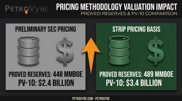
Then build low, mid, and high commodity price scenarios instead of one fixed number. A 2021 SEC filing illustrates why: switching from preliminary SEC pricing to a strip-pricing basis moved one company's proved reserves from 448 MMBoe to 489 MMBoe, and PV-10 from $2.4 billion to $3.4 billion. That's a billion-dollar swing from a pricing assumption alone.
Step 2: Build Production and Revenue Forecasts
Separate your production streams by reserve category. Proved Developed (PD) production follows a decline curve from existing wells with existing infrastructure, while Proved Undeveloped (PUD) production depends on assumed new wells drilled per year, tied to a type curve and development timeline.
Calculate revenue by multiplying forecasted production by realized prices, not benchmark index prices. Adjust for quality and location differentials, transportation deductions, and any hedging positions layered on top. Skipping the differential adjustment is a common way analysts overstate realized revenue by 5-15%.
Step 3: Model Costs, CapEx, and Cash Flow
Link production-linked operating expenses to a $/BOE or $/Mcfe basis so they scale with volume, not a flat annual number. Treat non-production costs like stock-based compensation as a percentage of revenue instead.
Forecast drilling and completion (D&C) capital expenditures tied directly to the new-well count you assumed in Step 2. Then roll PD and PUD cash flows into a single schedule, layering in corporate-level expenses and taxes.
Step 4: Discount Cash Flows and Calculate Valuation
Discount the aggregated cash flows to present value using a rate that reflects commodity price risk — not a generic WACC pulled from a comp set. Build the NAV bridge:
- Start with discounted asset-level cash flows
- Add non-core assets and undeveloped land value
- Subtract corporate liabilities and net debt
- Divide by share count (or partnership units) for NAV per share
Finish by stress-testing the model with sensitivity tables across your price scenarios, showing exactly how much valuation swings when commodity prices move.
The 4 Components of Oil and Gas Financial Modeling
Every O&G model, regardless of vertical, is built from four interdependent pieces. Get one wrong and the rest compound the error.
Revenue Projections
Revenue is a direct function of production volume multiplied by commodity price, two variables that are largely outside company control. A small shift in your price deck can swing valuation output, which is exactly why you model in ranges rather than fixed points.
Cost Estimation
Drilling, extraction, transportation, and refining costs vary by region and are rarely standardized across basins. Misclassifying production-linked costs versus fixed costs distorts margin forecasts and throws off cash flow timing across the entire model.
Production Forecasting
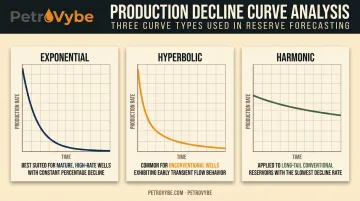
Decline curve analysis and new-well assumptions determine how long an asset generates cash flow before depletion. Industry guidance from SPE's Petroleum Resources Management System recognizes exponential, hyperbolic, and harmonic decline behaviors, and cautions that production forecasts depend on sufficient history and comparable operating conditions.
This is typically the single biggest driver of long-term model reliability: reserves, not revenue growth, underpin valuation here.
Valuation Metrics
The NAV model discounts asset-level cash flows to present value because there's no terminal value for a depleting asset. Your choice of discount rate and reserve category (PD vs. PUD vs. probable) shapes how conservative or aggressive your final output looks. Pick the wrong category and you've either overstated or buried real value.
The 4 Types of Oil & Gas Financial Models
Each vertical of the oil and gas industry functions like a different business, and each requires its own modeling approach. Applying one template across all four is a common, costly mistake.
| Vertical | Valuation Method | Key Driver |
|---|---|---|
| Upstream | NAV | Reserves & type curves |
| Midstream | DCF / Distribution Discount | Contracted fee revenue |
| Downstream | DCF / TEV-EBITDA | Crack spread margins |
| Integrated & Royalty | Sum-of-the-Parts / NAV | Segment mix or land ownership |
Upstream (Exploration & Production) Models
Upstream models are built around NAV methodology and are the most CapEx-intensive, commodity-sensitive vertical in the industry. They require specialized reserve data and engineering-validated type curves to be worth anything.
This is the exact model type used to underwrite direct natural gas development investments, where reserve categories and type curve accuracy drive investor returns. PetroVybe's finance team applies this approach to its South Texas and Gulf Coast Basin projects.
CFO Clayton Riddle built more than 70 upstream and midstream acquisition models earlier in his career at Odyssey Energy, advising CEOs and capital sponsors on deal viability. That underwriting discipline now shapes PetroVybe's own project-level models, including the $48MM proved reserves valuation independently verified for its Lavaca County assets.
Midstream (Storage & Transportation) Models
Midstream businesses function like utility companies: fee-based, contracted revenue with limited direct commodity exposure. Valuation typically uses DCF and Distribution Discount Models, with close attention paid to MLP structures and how those partnerships treat distributions.
Downstream (Refining & Marketing) Models
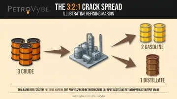
Downstream revenue and costs both track commodity prices, but through refining margins, often expressed as the crack spread. The EIA defines a 3:2:1 crack spread as three barrels of crude producing two barrels of gasoline and one barrel of distillate, a shorthand for refining profitability. These models rely on standard DCF and TEV/EBITDA multiples rather than NAV.
Integrated Majors & Royalty Companies
Integrated companies combine upstream, midstream, and downstream segments under one roof. Because each segment runs on a different economic engine, these companies are typically valued using Sum-of-the-Parts. Each segment is valued on its own method, then combined and reconciled for corporate items and net debt.
Royalty companies simplify this to land ownership: a non-cost-bearing share of production revenue valued through reserve-based NAV rather than SOTP.
Common Mistakes to Avoid When Modeling Oil & Gas Assets
Most modeling failures trace back to a handful of repeatable errors:
- Using a single commodity price scenario. Markets move, and your model needs to reflect that. Build low, mid, and high cases rather than betting everything on one number.
- Making unit conversion errors between barrels, cubic feet, and BOE. The 6:1 Mcf-to-Bbl conversion measures energy equivalence, and treating it as value equivalence silently skews production and revenue math.
- Forcing a standard DCF with terminal value onto an Upstream E&P company. Reserves deplete to an economic limit. A perpetuity terminal value doesn't belong on a finite asset base, which is exactly why the NAV approach exists.
Frequently Asked Questions
What are the 4 components of oil and gas financial modeling?
Revenue projections, cost estimation, production forecasting, and valuation metrics. Each depends on the others, so an error in one component compounds through the rest of the model.
What are the four types of oil and gas financial models?
Upstream (NAV-based), Midstream (DCF/utility-style), Downstream (margin-based DCF), and Integrated/Royalty (Sum-of-the-Parts). Each vertical's revenue mechanism dictates its valuation method.
What is a NAV model in oil and gas?
An asset-level discounted cash flow model with no terminal value, used mainly for Upstream E&P valuation. It discounts reserve cash flows to their economic limit rather than assuming perpetual growth.
Why can't you use a standard DCF model for E&P companies?
The terminal value assumption doesn't work for depleting, finite reserves. Reserves stop qualifying once production hits its economic limit, so a perpetuity overstates value.
What Excel skills are needed to build an oil and gas financial model?
Scenario and sensitivity tables (one- and two-variable data tables), TRANSPOSE and OFFSET functions, and careful unit conversion handling across Bbl, Mcf, and BOE.
How is oil and gas financial modeling different from other industries?
Commodity prices are uncontrollable, and assets deplete over time instead of growing indefinitely. Units like Bbl, Mcf, and BOE also require constant conversion discipline that most corporate models never touch.
Conclusion
Building an accurate oil and gas model comes down to three things: quality reserve data, correct unit conversions, and matching the valuation method to the vertical. Skip any one of those and the model looks fine until the numbers don't hold up under scrutiny.
Most failures stem from oversimplified price assumptions or misapplied valuation frameworks — like forcing a standard DCF onto a depleting Upstream asset instead of using NAV.
For investors evaluating direct participation in natural gas development, understanding these models is key to judging real return potential.
Firms combining in-house modeling expertise with independent third-party engineering validation offer added confidence that assumptions hold up. PetroVybe's South Texas and Gulf Coast Basin projects, for example, carry a $48MM PV-reserves verification backed by Chief Geophysicist Michael Stamatedes' 75.2% career well-selection success rate.