Most savings accounts compound daily, monthly, or quarterly. But understanding the continuous model matters because it reveals the underlying mechanic that drives wealth over decades: the frequency of reinvestment, not just the rate itself.
This guide breaks down the definition, the formula, and a few worked examples. We'll also connect the same compounding logic to real long-term wealth strategies, including how natural gas development investing uses reinvestment to scale returns over time.
Key Takeaways
- Continuous compounding produces the theoretical maximum growth rate through infinite reinvestment
- The formula FV = P × e^(rt) uses Euler's number (e ≈ 2.71828) instead of period counts
- Daily compounding gets close to continuous compounding in dollar terms
- In practice, it's a modeling tool, not a typical bank product feature
- This same principle powers long-term strategies like MOIC-driven passive income
What Is Continuous Compounding?
Continuous compounding is the mathematical limit of compound interest as the number of compounding periods per year approaches infinity. It comes directly from the standard compound interest formula:
A = P(1 + r/n)^(nt)
As n (the number of periods) grows toward infinity, this expression converges to:
A = P × e^(rt)
That constant, e, is Euler's number, roughly 2.71828. It isn't arbitrary. It emerges naturally from the limit itself, the same way pi emerges from circles.
University of Nebraska-Lincoln course materials demonstrate this convergence at a 7% rate:
- 1,000 compounding periods per year: a factor of 1.0725056
- 10,000 compounding periods per year: a factor of 1.0725079
- The continuous limit: a factor of 1.0725082
Continuous vs. Periodic: The Core Distinction
Periodic compounding pays interest at fixed intervals, annually, monthly, or daily. Continuous compounding assumes interest accrues at every possible instant, with no gaps between calculations.
A common misconception: continuous compounding equals daily compounding. It doesn't. Continuous compounding happens far more often than daily, but the numerical gap between the two is tiny.
At a 5% annual rate, for example, daily compounding produces a growth factor of 1.051267 versus continuous compounding's 1.051271, a difference of four ten-thousandths. We'll break down this gap further in the next section.
Who Actually Uses This Concept
Continuous compounding rarely shows up on a bank statement. Instead, it's a tool for:
- Bond yield conversions, translating between bank-discount, bond-equivalent, and continuously compounded rates
- Options pricing, most notably the Black-Scholes model
- Valuation modeling, where analysts discount future cash flows using exponential functions
Financial professionals and actuaries rely on it because exponential math behaves cleanly across any time interval, not because your checking account is compounding every microsecond.
Continuous Compounding Formula & How to Calculate It
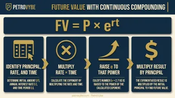
The core formula is:
FV = P × e^(rt)
Where:
- P = principal (starting amount)
- r = annual interest rate, as a decimal
- t = time, in years
- e = Euler's number (≈2.71828)
This comes from the same derivation logic covered above: start with A = P(1 + r/n)^(nt), let n approach infinity, and the expression collapses into e^(rt).
Calculating future value takes four steps:
- Identify your principal (P), annual rate (r), and time in years (t)
- Multiply r × t
- Raise e to that power (r × t)
- Multiply the result by P
Worked Example: Calculating Future Value
Say you invest $10,000 at a 9% annual rate, compounded continuously, for 10 years.
- r × t = 0.09 × 10 = 0.9
- e^0.9 ≈ 2.4596
- FV = $10,000 × 2.4596 = $24,596
That example shows continuous compounding's power over a long horizon. To isolate how compounding frequency alone affects returns, compare that same $10,000 at 15% for one year across different schedules. This side-by-side comes straight from Investopedia's own comparison:
| Frequency | Ending Balance | Effective Annual Return |
|---|---|---|
| Annual | $11,500.00 | 15.00% |
| Quarterly | $11,586.50 | 15.87% |
| Monthly | $11,607.55 | 16.08% |
| Daily | $11,617.98 | 16.18% |
| Continuous | $11,618.34 | 16.18% |
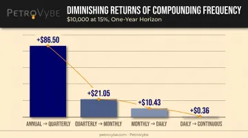
Notice the pattern: jumping from annual to quarterly adds $86.50. Jumping from daily to continuous adds just $0.36. That's the diminishing-returns effect in action, according to Investopedia's continuous compounding breakdown. More frequency always helps, but each additional increment matters less than the last.
Reversing the Formula: Present Value
To discount a future cash flow back to today's dollars, flip the exponent's sign:
PV = FV × e^(-rt)
If you need $1 in one year and the continuous rate is 6%, present value comes out to roughly $0.9417. This discounting approach underpins standard bond and derivatives pricing models.
Continuous vs. Periodic Compounding: Key Differences
Increasing compounding frequency, annual to quarterly to monthly to daily to continuous, increases your effective annual rate. But each step forward buys you less than the one before it.
Using the same $10,000 at 15% example above:
- Annual → Quarterly: +$86.50
- Quarterly → Monthly: +$21.05
- Monthly → Daily: +$10.43
- Daily → Continuous: +$0.36
The pattern is unmistakable: gains shrink fast as frequency rises. By the time you're comparing daily to continuous, you're arguing over pocket change on a five-figure balance.
This is why continuous compounding works best as a benchmark: a reference point rather than a practical goal. It represents the theoretical ceiling for a given nominal rate. Every periodic compounding method, whether it's your savings account or a bond yield calculation, can be measured against that ceiling to see how close it gets.
For most practical financial decisions, daily compounding already sits close enough to that ceiling that chasing continuous compounding adds no meaningful value.
Is Continuous Compounding Realistic? Applications & Limitations
Here's the direct answer: no real-world bank, fund, or loan literally compounds continuously. Doing so would require infinite calculations executed in zero time, which no operational system can perform. Continuous compounding exists as a mathematical idealization, useful for modeling, not as a product feature.
Where It Genuinely Gets Used
- Options pricing (Black-Scholes model): The Black-Scholes formula uses the continuously compounded risk-free rate to discount the strike price, per CFA Institute research
- Bond yield conversions: Analysts convert between bank-discount rates, bond-equivalent yields, and continuously compounded rates for apples-to-apples comparisons
- Exponential growth and decay modeling: Population models, radioactive decay, and other natural exponential processes use the same e^(rt) structure
- Continuous discounting in valuation: Advanced valuation models sometimes discount cash flows continuously for mathematical cleanliness across any time interval
Key Limitations
- It assumes uninterrupted, volatility-free reinvestment, which doesn't reflect how real markets behave
- Applying it to consumer products like CDs or savings accounts can overstate return expectations
- It's a rate convention for modeling, not proof that any institution credits interest at infinite instants
Continuous compounding remains a precise mathematical tool that financial professionals lean on for pricing and valuation, not a feature you'll find advertised on a savings account rate sheet.
Why the Compounding Mindset Matters for Long-Term Wealth
Strip away the formula, and continuous compounding teaches one lesson: reinvested returns accelerate growth faster than returns you pocket and walk away from. Whether that reinvestment happens annually, daily, or theoretically every instant, the principle behind it is what separates linear savers from long-term wealth builders.
That same logic applies well beyond interest-rate math. In real asset classes, reinvesting cash flow into new development, workovers, and acquisitions can scale output over time instead of relying on a single static return rate.
This is exactly the model that PetroVybe, a Texas-based natural gas development company, applies to upstream energy projects. Rather than banking on one well's performance, PetroVybe's growth framework, known internally as PROTECT and SCALE, reinvests operating cash flow into:
- New well development, guided by geological and production data
- Targeted workovers on existing legacy assets
- Strategic acquisitions of producing properties
The company describes this as "stacking wells like compounding interest": each new well's cash flow helps fund the next round of development, creating a self-reinforcing growth cycle rather than a one-time outcome.
That approach has produced measurable results, including growth from zero to roughly 1,300 BOEPD across nearly 400 producing wells on 58,000 acres, alongside a third-party engineered $48 million proved reserves valuation.

PetroVybe targets a 10-year MOIC of approximately 2.2x to 5.8x with a projected ~26% IRR, structured for accredited investors seeking tax-advantaged, inflation-resistant passive income beyond traditional stocks and bonds.
It's the same principle as e^(rt), applied to physical assets instead of a bank ledger: reinvest the output, and growth compounds rather than stays flat.
Frequently Asked Questions
What is the continuous compounding rate?
The continuous compounding rate is calculated using r_continuous = ln(1 + r), representing the return you'd need assuming infinite compounding frequency. This formula converts a standard effective rate into its continuous equivalent.
How do you calculate future value with continuous compounding?
Use FV = P × e^(rt). You need four inputs: principal (P), annual rate as a decimal (r), time in years (t), and Euler's number (e ≈ 2.71828).
Is continuous compounding realistic?
Continuous compounding is a theoretical construct used in financial modeling, options pricing, and bond yield conversions rather than a product banks offer. Daily compounding comes close enough in practice that the dollar difference is negligible.
What is the difference between continuous and discrete compounding?
Discrete compounding applies interest at set intervals, daily, monthly, or annually. Continuous compounding assumes interest accrues at every possible instant, with no gaps between calculations.
Does continuous compounding mean the same thing as daily compounding?
No. Continuous compounding occurs far more frequently than daily compounding in theory. In practice, though, the dollar difference between the two is usually just a few cents to a few dollars, as shown in the $10,000 example above.
Why does the continuous compounding formula use Euler's number (e)?
Because e emerges mathematically as the limit of (1 + r/n)^n as n approaches infinity. It's the natural constant that falls out of modeling unlimited compounding frequency, not an arbitrary choice.